Dynamic Co-attention Network
Overview
- Similar to BiDAF, this paper introduces an attention layer (Co-attention) that flows both ways.
- However, this is a 2 layer attention (we compute attention on top of existing attention layers).
Architecture
Assume we’ve the context hidden states \(c_1,....,c_N \in \mathbb{R}^{l}\) and question hidden states \(q_1,....,q_M \in \mathbb{R}^{l}\). First, we apply a linear layer with tanh non-linearity to the question hidden states to get the projected question hideen states (q’).
\[\begin{align*} q'_{j} = tanh(Wq_j + b) \in \mathbb{R}^l \end{align*}\]Next we add sentinel vectors \(c_{\phi} \in \mathbb{R}^l\) and \(q_{\phi} \in \mathbb{R}^l\) which are both trainable vectors.
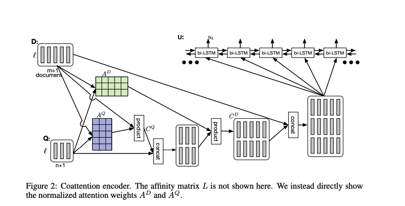
First Level Attention Layer
Similar to the BiDAF, we compute the affinity matrix (L) and C2Q attention layer (ai) and Q2C attention layer (bj).
Second Level Attention Layer
The advantage with DCN, is that we’ve a second-level attention layer. This is an attention layer on top of the first-level attention layer.
\[\begin{align*} s_{i} = \sigma_{j=1}^{M+1} \alpha_j^ib_j \in \mathbb{R}^l \end{align*}\]Output
Finally, we concatenate the second-level attention layer outputs si with the first level C2Q attention outputs ai, and feed the sequence with a BiLSTM. We then return the final hidden state.
\[\begin{align*} { u_1, ..., u_N} = biLSTM({[s_1;a_1],....[s_N;a_N]}) \end{align*}\]Results
| Paper | EM | F1 |
|---|---|---|
| Dynamic Co-attention Networks | 65.4 | 75.6 |
| Match LSTM | 59.1 | 70.0 |

Kaushik Rangadurai
Code. Learn. Explore